How To Apply Woven Mat Textrue To Chart In Excel

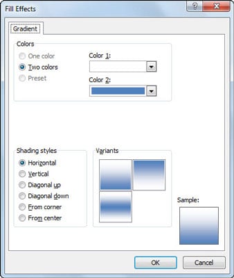
Excel 2010 Add Or Change A Gradient Texture Or Picture Fill Youtube

Microsoft Excel Tutorials How To Format Pie Chart Segments

Link Left And Right Textboxes And Remove Borderlines From Both Textboxes Then Apply Woven Mat Youtube
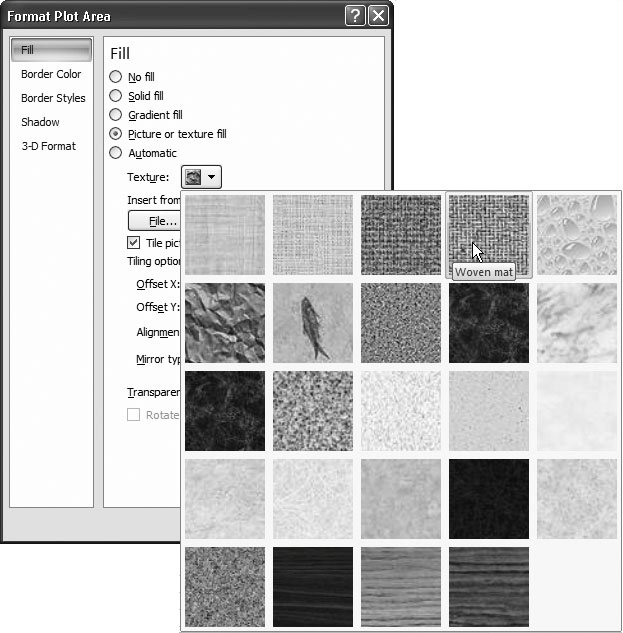
How To Apply The Woven Mat Texture Fill In Excel
Https Www Ikenotech Com Wp Content Uploads 2019 02 Ex2016 Independentproject 3 4 Instructions Pdf
Section 18 4 Formatting Chart Elements Excel 2007 C The Missing Manual

Apply the woven mat texture fill to the patio and furniture slice.
How to apply woven mat textrue to chart in excel.

How To Apply The Woven Mat Texture Fill In Excel
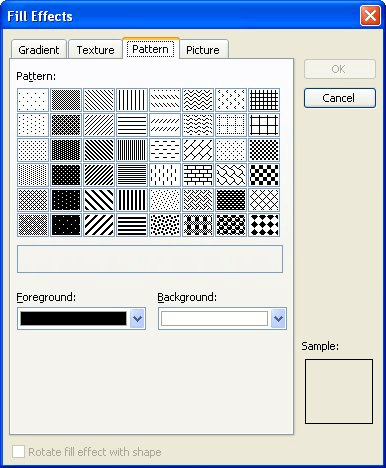
How To Apply Fill Colors Patterns And Gradients To Cells In Excel 2010 Dummies

Weaved Place Mats Paper Weaving Weaving For Kids Weaving Art

Reversible Knitting 50 Brand New Groundbreaking Stitch Patterns Preview Knitting Stitch Patterns Stitch

Marvel Cinematic Universe C2c Graphigan Pattern Queen Size Etsy In 2020 Superhero Blanket Crochet Patterns Free Blanket Blanket Knitting Patterns

Inspired By Cobblestone Streets And Stone Pathways Scattering The Design Makes The Composition Seem Almost Naturally Occ Carpet Tiles Yellow Decor Wall Design

Angel Blanket Home Decor Blanket Decor

Beach Hut Blanket Crochet Pattern By Rachele Carmona Knitting Patterns Loveknitting Blanket Pattern Crochet Blanket Patterns Crochet Patterns

24 X 34 Navy Tan Gold Rope Rug Nautical Decor Tightly Knotted Doormat Inside Or Outside Mat Beach House Decor Lovers Knot Nautical Rugs Rope Rug Rugs

Terrazzo Afghan In 2020 Afghan Pattern Mosaic Patterns Terrazzo

Multicolor Table Mat Crochet Free Pattern Knit Blankets Are One Of Our Favorite Weaves That We See In Our In 2020 Crochet Patterns Crochet Crochet Stitches Patterns

Bound Rosepath More Yarn And Time Please Warped For Good Weaving Loom Projects Weaving Yarn Weaving Patterns

Your Place To Buy And Sell All Things Handmade Decorative Pieces Large Centerpiece Woven

Textured Weave Bath Mat Mustard Yellow Home All H M Us Yellow Bathroom Rugs Bathroom Rugs Bath Rugs

Block Design Rug Free Crochet Pattern Rug Pattern Crochet Rug Crochet Patterns

Evil Eye Boho Doormat In 2020 Door Mat Eye Decor Custom Doormat

Beachcrest Home Austell Hand Braided Navy Beige Indoor Outdoor Rug Wayfair Co Uk Outdoorrugs Austell Hand In 2020 Handgefertigte Teppiche Haus Am Meer Lila Teppich

Hanlontown Area Rug Boutique Rugs Rugs Area Rugs Hand Weaving
Https Encrypted Tbn0 Gstatic Com Images Q Tbn And9gcrtsbxsdjo0tptvdllg152latwq4vegmsie4otlgnp7uxdwtb58 Usqp Cau
Source : pinterest.com
